Quantification of cellular morphology using Deep Learning
Published:
Introduction
The machine learning/Artificial intelligence field has made quantum leaps in the past few years. The advent of AlphaFold, stable diffusion (e.g. the DALL-E model) and chatGPT are a few recent examples. Deep Learning is a branch of machine learning that uses large neural networks. These are inspired by biological neural networks in that they have a set of inputs and outputs, with the layers in between them being defined by a set of parameters which form a representation that maps given inputs to their outputs. How is this learning? The set of parameters are learned by running the model on a training dataset. When the model is applied to an unseen dataset during runtime, the accuracy of the model is dependent on whether the learned parameters remain to faithfully predict the correct output. One category of deep learning is for image recognition. For those who want to learn more, I recommend the fastai course by Jeremy Howard.
In this post I use a machine learning model for cell segmentation. Next, I combine cellProfiler (an open source image analysis software) with an implementation of a deep learning model (a resnet50) in PyTorch. This model is trained from scratch to morphologically classify cells after drug treatment. During this optimisation problem the model learns important features about cellular morphology that should temporally distinguish cells post treatment. This is termed a weakly supervised learning problem because we are creating artificial labels for our data, e.g. timepoints post drug treatment, in the hope that this will be sufficient for the models inference. All of the aforementioned code is dispatched to a linux high performance computer cluster (HPC) using bash scripts. Because I performed this work at a pharmaceutical company, I am not going to make the data available and will redact some of the data identifiable code. This work was also performed a couple years ago. It was exciting at the time and I am writing up what I learnt from this experience despite the method now being sort of outdated! For instance, I believe cellprofiler has integrated machine learning based segmentation methods and there is a whole consoritum for cell painting established by Anne Carpenter you can check out. Neverless, I learned a lot of programming skills applied to image analysis during this work.
An overview of the data
In this imaging experiment four dyes were used to monitor cell death after treatment with a chemotherapeutic: the nuclei dye Hoechst; the membrane dye cell tracker green; the early apoptotic dye annexin, and the late apoptotic dye propidium iodide. Three replicates of cells were treated with seven drug concentrations (+ a no drug control) and imaged at 4 hrs, 8 hrs, 16 hrs, 24 hrs, 48 hrs and 72 hrs using a confocal microscope set to aquire nine fields of view (FOV) per sample across six Z-stacks. Each FOV contains a total of five channels (i.e. including the unstained brightfield channel). Therefore, we have a total of 12,960 image slices (8 x 6 x 9 x 6 x 5 x 3). This is the following outline of the project given the aforementioned information:
- STEP 1: Perform a max-Z projection across the six Z-slices.
- STEP 2: Perform cell segmentation.
- STEP 3: Implement a resnet50 model and perform feature extraction (i.e. open up the neural network to extract the important representation it has created).
- STEP 4: Perform principal component analysis (PCA) on these feature representations to visualise how well the prediction weights separate cells across timepoint and concentration.
STEP 1: Creating a file structure
The representation of each image as six Z-stacks produces a high resolution image because it captures cells that may lie in different planes (e.g. if they have different morphologies). To collapse the Z-stacks into one high resolution image that faithfully represents that FOV we can take an average of each of the six pixels or the maximum value. This can be performed using cellProfiler or using a Python script. Because there was no difference between the quality of the different Z-planes I just chose the middle image. I guess if you had cells growing in different planes, such as suspension cells, averaging the Z-stack would be more useful here.
The first step is to create a file structure on my /scratch/hpc/ node by transferring and organising the image files located on the network drive. The FOV, Z-stack and well number of each image file is extracted using regex (check out this tool and this metadata used to create a folder structure of well > FOV > Z-stack per channel for storing the images.
For succintness I have only included the code needed to retrieve the middle Z-plane of the brightfield channel because the code remains the same for the other channels (This could probably have been better written). A conda environment should be created prior with all the installed packages that are needed. If I don’t know what packages I need in advance, I find it easier to create a conda environment and install conda packages individually rather than creating a .yml file.
# Import packages
import os
import glob
from skimage import io
import numpy as np
import matplotlib.pyplot as plt
import re
%matplotlib inline

# Retrieve images using wildcard syntax
img_file_list = sorted(glob.glob('/hpc/scratch/hdd2/fs541623/Pre_processed_Images/*/*'))

# Save each middle Z-plane (Z3) to the appropriate directory
for i, n in enumerate(img_file_list):

    # Get Timepoint
    timepoint_re = re.compile(r'\d+hrs_R\d')
    timepoint = 'Time_' + str(timepoint_re.findall(os.path.dirname(n))[0])

    # Get Well Number
    Well_re = re.compile(r'W\d{2}(\d+)')
    Well_no = 'Well_' + str(Well_re.findall(str(n))[0])

    # Get Field Number
    Field_re = re.compile(r'F\d{3}(\d)')
    Field_no = 'Field_' + str(Field_re.findall(str(n))[0])

    # Get Channel Number
    Channel_re = re.compile(r'C(\d)')
    channel_no = 'C' + str(Channel_re.findall(str(n))[0])
    print(f'channel number : {channel_no}')

    # Paths to Brightfield and Single Channel Images
    path_C1 = os.path.join(output_dir, timepoint, Well_no, 'Brightfield')
    path_B = os.path.join(output_dir, timepoint, Well_no, 'Nuc')
    path_G = os.path.join(output_dir, timepoint, Well_no, 'Cyt')
    path_pi = os.path.join(output_dir, timepoint, Well_no, 'PI')
    path_AnnexinV = os.path.join(output_dir, timepoint, Well_no, 'AnnexinV')


    # Save Brightfield Channel - middle Z // Repeat for each channel
    if 'Z003C1' in str(n):
        img_C1 = io.imread(n)
        print(n)

        # Create New directory for each Timepoint and
        # Well if it already doesn't exist
        if not os.path.exists(path_C1):
            os.makedirs(path_C1)

        # Name flile using the regex attracted metadata
        Brightfield_name = f'{timepoint}_{Well_no}_{Field_no}_{channel_no}.tif'
        io.imsave(os.path.join(path_C1, Brightfield_name), img_C1)
        print('--------------------------------C1 saved----------------')
The above script was dispatched to the HPC cluster using the following bash script. Bash scripts (.sh) can be written in visual studio code or notepad (just ensure that the settings are Unix(LF) and UTF-8 in order to correctly handle end of line characters).
#!/bin/bash

#SBATCH --job-name=pre_processing
#SBATCH --time=1:00:00
#SBATCH --nodes=1
#SBATCH --ntasks=1
#SBATCH --output=pre_processing%A.out
#SBATCH --error=pre_processing%A_%a.err
#SBATCH --cpus-per-task=6
#SBATCH --mem-per-cpu=20
#SBATCH --partition=cpu

# Set Environment
module purge
module load anaconda3
source activate conda environment

# Run pre_processing script
# Supply your own input file and output directory in single brackts
python /hpc/scratch/hdd2/fs/CellToxExp/STEP1_Pre_processing_CellTox/pre_processing/STEP1_Pre_Processing.py 'Input' 'Output'
STEP 2: Cell Segmentation
In this experiment the aim is to extract morpological information from single cells. Each cell will be used as an input into the deep learning model. This requires segmentation of the cells using the CellMask green stain in order to isolate each individual cell and create single cell cropped images for every field of view per condition.
Cell segmentation can be performed using arbitary pixel threshold methods (e.g. otsu) or machine learning. Cellpose worked well for this dataset and the paper shows its applicability across a variety of cell types. The algorithm is based on a neural net trained to predict pixel values belonging to cells and their spatial gradients. The latter uses a heat diffusion model, where predicts the spatial gradients radiating from the centre of a cell. All the pixels that flow to this centre are classified as being from the same cell.
Cellpose can be run from a GUI cell pose GUI, but given that we have a large dataset we will run it from the command line using bash scripting. We will use the cellmask channel to segment the cell. The output of cellpose is a series of unique pixel values (termed cell masks) corresponding to each cell in the segmented images (i.e. each cell is a different grayscale pixel value). We can use this mapping to isolate individual cells and extract features such as the cell count and even more specific statistics such as cell size, roundness and eccentricity. The cells touching the border of the image are excluded because they would skew the overall statistics.
#!/bin/bash

#SBATCH --job-name=CellposeSegmentation270421
#SBATCH --time=20:00:00
#SBATCH --nodes=1
#SBATCH --ntasks=1
#SBATCH --output=Cellpose_Segmentation_%A.out
#SBATCH --error=cellpose_Segmentation_%A_%a.err
#SBATCH --cpus-per-task=6
#SBATCH --gpus=1


module purge
module load anaconda3

# Load enviornment where cellpose has been installed
source activate conda environment


# Run cell Segmentation
for image in /hpc/scratch/hdd2/fs/Pre_processed_Images/*/*/Cyt; do
	python -m cellpose --dir $image --use_gpu --pretrained_model cyto --chan 2 --diameter 0 --save_png
done
STEP 3: Model pre-processing
One of the most useful pieces of information to deduce from this data is cell death over time and across the different concentrations. To extract these statistics we can use the open source image analysis software cell profiler. As we have thousands of images we can run the pipeline as a slurm job as long as cellprofiler is installed on your HPC cluster. In the below code I crop each individual cell from each brightfield image using the corresponding cell mask and then make each image the same size. Firstly, I loop through the saved pixel identity maps for each image and create a list of these pixel values. I then find the path to the corresponding brightfield image using the metadata from the filename of the pixel identity maps and crop each individual cell in each brightfield image using its corresponding pixel identity. The get_cropped_obj function loops through the pixel identity map list, converts the grayscale mask into a binary mask (1 - white/cell, 0 - black), identifies the x and y centre coordinates of the mask and applies a guassian blur (more details below) and uses this to save 200x200 pixel single cell images.
I thought applying a guassian blur to the mask was necessary when cropping indivudal cells as otherwise the cell’s edges became jagged and not ‘cell like’. Finally, I save each individual cell so that it aligns to the statistics created by cellprofiler. These single cell crops will be used as inputs into a resnet50 deep learning network. The aforementioned pre-processing involving cropping individual cells and centering them in a 200x200 image was important because image classifiers tend to focus on the centre of the image.
# Packages
from skimage import io, exposure
import pandas as pd
import numpy as np
import os
import glob
import matplotlib.pyplot as plt
import re
import cv2

##### Define your own directories #####

# Get CSV for each timepoint/well
def main(well_csv_list, re_time, re_well, BF_path, output):
    for csv in well_csv_list:
        print(f'--current csv: {csv}--')

        # BF_file and Obj csv file located in different dir; use csv to match each obj to correct BF_image
        df = pd.read_csv(csv); BF_files = df.iloc[:, df.columns.get_loc('FileName_BF')]

        # For each csv (timepoint/well) split csv into different FOV (1-9)
        # Reset field number for each csv file i.e. well
        for f, field in enumerate(pd.unique(BF_files)):

            # Locate correct BF_image using metadata extracted from csv file
            time = re_time.findall(str(field))[0]; well = re_well.findall(str(field))[0]
            BF_file = f'{BF_path}/{time}/{well}/Brightfield/{field}'

            # Split df on FOV; get centre coordinates for each obj
            df_field = df[df['FileName_BF'].isin([field])]

            # Get Image masks for every FOV in Well
            mask_path = f'{mask_dir}/{time}/{well}/{field}/FilteredCyt*'
            img_list=sorted(glob.glob(mask_path), key=os.path.getctime)
            img_masks = io.imread_collection(img_list)

            # Centre crop all objects & Save to new CentreCrops/Timepoint/Well/*
            output_dir = os.path.join(output, time, well)

            for obj in range(0,len(df_field)):
                obj_filename = f'{time}_{well}_Field_{f+1}_obj{obj}.tif'
                cropped_img = get_centre_crop(df_field, BF_file, obj, img_masks[obj])
                save_crop(obj_filename, cropped_img, output_dir)

            # Update field number
            print(f'outer -----------Object: {obj} for field: {field} {f+1}successfully cropped-----------')

    return 0


# Centre Crop Cells
def crop_img(df, BF_file, obj_number, mask):

    # Load Image
    BF_img = skimage.io.imread(BF_file).astype('float')/255

    # Get Coordinates
    centre_X = int(df.iloc[obj_number, df.columns.get_loc('Location_Center_X')])
    centre_Y = int(df.iloc[obj_number, df.columns.get_loc('Location_Center_Y')])

    # Crop using centre
    y2, y1, x2, x1 = int(centre_Y+100), int(centre_Y-100),  int(centre_X+100), int(centre_X-100)
    cropped = BF_img[y1:y2, x1:x2]

    return (cropped, centre_X, centre_Y)


# Save a pseudo RGB image to timepoint/well dir so that input images are compatible with resnet50
def save_crop(file, img, output_dir):
    if not os.path.exists(output_dir):
        os.makedirs(output_dir)
    grayscale_stack = np.dstack([img, img, img])
    skimage.io.imsave(os.path.join(output_dir, file), grayscale_stack)

    return 0

# Apply a guassian blur to binary mask and use this to generate single cell crops
def get_centre_crop(df, BF_img, obj_number, mask):
    mask_blurred  = cv2.GaussianBlur(mask,(3,3),0)
    mask_large=np.where(mask_blurred>0, BF_img, 1)
    mask_large_blurred = cv2.GaussianBlur(mask_large, (11,11),0)
    img=mask_large_blurred.astype('float')/255
    img=((img*BF_img)*255).astype('uint16')
    return (crop_img_test(df, img, obj_number))


if __name__ == '__main__':

    # Input/output dir
    input_obj_csv = sorted(glob.glob('{location_of_cropped_cells_from_cell_profiler}/*/*/FilteredCytObj.csv'), key=os.path.getctime)
    output_path = '{output_dir}'
    BF_path = '{dir_for_brightfield_images}/Pre_processed_Images'

    # Compile Regex; pass into main to extract img metadata to create filenames
    re_time = re.compile(r'(Time_\d+hrs_R\d)')
    re_well = re.compile(r'(Well_\d+)')

    # Save centre cropped cells for each img in each timepoint/well
    main(input_obj_csv, re_time, re_well, BF_path, output_path)
STEP 4: The model
Now we have ~million single cell crops of the same size representing different timepoints and drug dosages. I will leave an explanation of the architecture of a resnet50 model for another post. In this case I wrote out a resent50 from scratch using the original paper. As a summary, image classifiers are composed of different kernels/channels (just a small matrix that represents a function e.g. the guassian blur mentioned above is an example of a kernel) that ‘detect’ features of the input image. In a deep learning network these kernels are not predefined, rather they are randomly initialised and then optimised (as they are just matrices of numbers) to identify features that most faithfully predict the correct output. As a simple example, the final weights may ‘learn’ that a higher treatment dose correlates to rounder cells. You would hope that running such a large complicated model would not result in this simple mapping (because we could have deduced this from cellprofiler) but rather identify more complicated non-linear mappings.
Lets ignore the resnet50 model for now, but focus on how to process the input data of millions of cells for input into the model. Here the fastai library really comes in handy for doing most of the heavy lifting. First, we load the image files using a fastai built-in function. Next, we need to create a series of labels for our data using regex and our image filenames to get a unique number of labels and a label count (classes). Then we randomly shuffle the data and split it 80% and 20% for the training and testing set respectively. Finally, I encode the filenames with a unique label (where 1 is the label e.g. {time_0:1, time_1:0, time_2:0} etc) that will represent the output layer of the neural network. To decode these labels I create a function that looks up the key of that given label (e.g. time_0 in this case).
from fastai import *
from fastai.data.all import *
from fastai.vision.data import *
from fastai.vision.core import *
from fastai.vision.all import *
from torchvision import transforms
from torch_lr_finder import LRFinder
import torch.optim.lr_scheduler as lr_scheduler
import torch.utils.data as data
from torch import nn, optim
from sklearn.preprocessing import MultiLabelBinarizer, OneHotEncoder
import re
import os
import glob
from skimage import io, color, img_as_float32, img_as_uint
import random
import numpy as np
import PIL
import glob
import gc
from torch.optim.lr_scheduler import _LRScheduler
from sklearn.metrics import fbeta_score
import sys
import builtins
import os

print('----------------------running script---------------')

# Fetch single cell crop paths
fnames = get_image_files('/hpc/scratch/hdd2/CellProfilerFeatureExtraction/CP_Cropped_Cells')
path_glob = glob.glob('/hpc/scratch/CellProfilerFeatureExtraction/CP_Cropped_Cells/*/*/*/*')
path_img = '/hpc/scratch/CellProfilerFeatureExtraction/CP_Cropped_Cells'

# Extract labels from filenames and identify total number of unique labels for the output layer
def label_func(fname):
    return (re.match(r'.*(Time_\d+hrs).*(Well_\d+).*', fname.name).groups())

labels = np.unique(list(zip(*(set(fnames.map(label_func))))))
label_n = len(np.unique(labels))
classes=len(labels)

# Encode the 'human' labels
labels_encoder = {metadata:l for l, metadata in enumerate(labels)}
def label_encoder(fname):
    time, well = re.match(r'.*(Time_\d+hrs).*(Well_\d+).*', fname.name).groups()
    return labels_encoder[time], labels_encoder[well]

# Decodes label for human interpretation
def label_decoder(labels):
    label_array=np.array(list(labels_encoder))
    idx = np.array(labels).astype(int) > 0
    return label_array[idx]

# Randomly shuffle the data and split into 80% and 20% train and validation sets
indxs = np.random.permutation(range(int(len(fnames))))
dset_cut = int(len(fnames)*0.8)

# Split into train & val
train_files = fnames[indxs[:dset_cut]]
valid_files = fnames[indxs[dset_cut:]]

## Get label encodings for each image
train_y = train_files.map(label_encoder)
valid_y = valid_files.map(label_encoder)
Building a neural network in PyTorch requires a dataset class. There is the base class provided by PyTorch, but this didn’t work well with my single cell cropped images so I created a new Dataset class that inherited from the base class. When I create an input image I apply a transformation (in this case a resize to 224x224 image but it could be a shear or other transformation) and associate each image with a label. I modified the getitem attribute to associate each image with its corresponding label and then format the my single channel grayscale images in the correct RGB tensor format for PyTorch.
Next, we use the DataSet class to create training and validation datasets and finally training and validation iterators based on these datasets. The model will take 16 images at a time and won’t shuffle them because we have already done that. I will explain more about how to create a resnet50 model in PyTorch in a separate post, but the resent50 has been out for ages! So expect to find lots of explanations online.
## Dataset
class Dataset(torch.utils.data.Dataset):
    def __init__(self, x, y):
        self.x = x
        self.y = y
        self.transform = transforms.Resize(224)

    def __len__(self):
        return len(self.x)

    def __getitem__(self, idx):
        img = img_as_float32(Image.open(self.x[idx]))
        out = np.zeros((1,14), int) # TO DO : refactor
        out[[0,0], np.array(self.y[idx])] = 1
        return (self.transform(torch.tensor((img[None]))), torch.tensor(out, dtype=float).squeeze())


## Create Datasets
train_ds = Dataset(train_files, train_y)
valid_ds = Dataset(valid_files, valid_y)


#dataloaders
train_iterator = data.DataLoader(train_ds, batch_size=16,shuffle=False, pin_memory=True, num_workers=64)
valid_iterator = data.DataLoader(valid_ds, batch_size=16,shuffle=False, pin_memory=True, num_workers=64)
When I done this I trained the model from scratch to predict time and dose after treatment. For predicting these two ‘weak’ labels the model achieved an accuracy of ~60%. Considering two labels were being predicted I thought this was a pretty good win. The below code defines some parameters for the model. In summary, we define the model to run for a specified set of training loops. At each training cycle, we optimise the models weights using the Adam optimiser gradient descent algorithm and a specified learning rate. The learning rate is dynamic in order to minimise overshooting the loss functions minima.
model = resnetmodel(channels=[64,128,256,512], n_blocks=[3,4,6,3])

lr, epochs, bs = 3e-5, 10, 8
device = torch.device('cuda' if torch.cuda.is_available() else 'cpu')

# Scheduler
params = [
        {'params':model.model_stem.parameters(), 'lr': lr/10},
        {'params':model.res_layer1.parameters(), 'lr': lr/8},
        {'params':model.res_layer2.parameters(), 'lr': lr/6},
        {'params':model.res_layer3.parameters(), 'lr': lr/4},
        {'params':model.res_layer4.parameters(), 'lr': lr/2},
        {'params':model.linear.parameters()}]


# Model will use an Adam optimiser for gradient descent
# Learning rate decreases at each layer to prevent overshooting the loss functions minima
optimizer = optim.Adam(params,lr=lr)
total_steps = epochs * len(data_iterator) # epochs * number of batches
max_lr = [p['lr'] for p in optimizer.param_groups]
scheduler = lr_scheduler.OneCycleLR(optimizer, max_lr, total_steps)

# Binary cross entropy (BCE) loss function evaluates actual target vs probability of output
loss_func = nn.BCEWithLogitsLoss()
model = model.to(device)
loss_func = loss_func.to(device)
The most useful part to do now is to derive biological insight from these predictions. We can identify what is seperating these different treatment groups by opening up the networks layers and extracting the features that predict the correct treatment group 60% of the time.
To extract the models embedding I focus on the final fully connected layer of the model, which has the dimension [0,2048]. I load the optimised weights generated from training and run the model without updating of the models weights - I purely just want to see what the final layer of the network is. My model (see separate post) is set up to save the channels of the fully-connected layer. I concatenate all the embeddings from each batch of images fed to the model and save these alongside the ground truth label and the predicted label in a pickle file.
print('loading weights')
model.load_state_dict(torch.load('/hpc/scratch/hdd2/fs541623/Bash_scripts/resnet50-scratch-p5.pt'))

data_iterator = data.DataLoader(data_ds, batch_size=16,shuffle=False, pin_memory=True, num_workers=64)

print('get_representations')

model.eval()

def get_representations(loader):

    count = 0
    embeddings = np.zeros(shape=(0,2048))
    predictions = np.zeros(shape=(0,14))
    labels = np.zeros(shape=(0,14))

    with torch.no_grad():
        for (x,y) in iter(loader):

            x = x.to(device)
            y_pred, features = model(x)
            y_pred = torch.sigmoid(y_pred) > 0.5

            predictions = np.concatenate((predictions, y_pred.cpu()))
            labels = np.concatenate((labels, y.cpu()))
            embeddings = np.concatenate([embeddings, features.detach().cpu()], axis=0)

            if (count %100000) == 0: print(f'Embeddings from 100000 extracted')
            count += 1

    return embeddings, predictions, labels

embeddings, predictions, labels = get_representations(data_iterator)

print('writing pickle file')
with open('representations_copy_full_3.pkl', 'wb') as f:
    pickle.dump([embeddings, predictions, labels], f)
STEP 5: Results
Here is where we hopefully gain some biological insight from arduous data pre-processing and modelling we’ve done. I am going to discard the cellprofiler features for now (but these could be concatenated with the features from the deep learning network) and show how well the features we extracted solely from our resnet50 separate treatment groups using principal component analysis (PCA). PCA baisically summarises these high dimensional data by identifying the most important features that ‘explain’ the variance between data-points. The below code reads in the representations we extracted, converts their labels and predictions to a dataframe, removes features that have zero variance, and selects the top 800 features that vary the most across the representations. These are then used to run PCA.
## Load X, predictions, and truth labels
x,y,z = pd.read_pickle(r'/hpc/scratch/hdd2/fs541623/Bash_scripts/representations_copy_full_3.pkl')

## Extracts human readable labels from models final layer
def get_labels(one_hot):
    labels= list()
    for i in one_hot:
        label = label_decoder(i)
        labels.append(label)
    return labels

## Convert from one hot to words
predictions = get_labels(y)
ground_truth = get_labels(z)
df1 = pd.DataFrame(predictions)
df2 = pd.DataFrame(ground_truth)

## Remove zero variance features using sklearn
from sklearn.feature_selection import SelectKBest
from sklearn.feature_selection import chi2
X_new = SelectKBest(chi2, k=800).fit_transform(x, y)
df3 = pd.DataFrame(X_new)

## colnames for features
df3.columns = [('Feature_' + str(i))  for i in range(1, df3.shape[1]+1)]
df1 = df1.rename(columns={0:'Time_prediction', 1:'Concentration_prediction'})
df2 = df2.rename(columns={0:'Time_label', 1:'Concentration_label'})

## Concatenate Dataframe on rows
concat = pd.concat([df3, df1, df2], axis=1, keys=['X','pred', 'truth'])

## flatten multidimensional dataframe for plotting
concat.columns = [(str(col[1])) for col in concat.columns.values]

## Run PCA ##
pca = PCA(n_components=20)
pca_result = pca.fit_transform(df3)
print('Variance PCA: {}'.format(np.sum(pca.explained_variance_ratio_)))
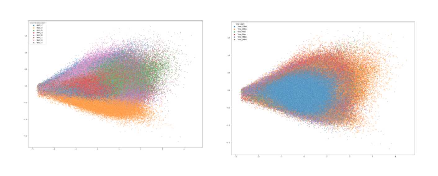
Below is a PCA plot where each dot represents a single cell and is coloured separtely by timepoint (Right) and concentration (Left). As expected, drug dose has a greater effect in separating single cells than time after treatment. The greater the difference in drug dose the larger the separation between groups (e.g. orange and purple coloured groups). This is just a starting point for exploring the models feature maps and theres lots more that could be done if I had more time, including combining the cellprofiler features with the deep learning extracted features. Regardless, I hope that this post has been a good introduction to how one might process high throughput imaging data, especially the pre-processing needed for modelling.
## PCA plot labelled by concentration
plt.figure(figsize=(20,15))
sns.scatterplot(pca_result[:,0], pca_result[:,1], hue=df2['Concentration_label'], s=10, alpha=0.9)
plt.savefig('pca_plot_concentration_label.png')

## PCA plot labelled by time
plt.figure(figsize=(20,15))
sns.scatterplot(pca_result[:,0], pca_result[:,1], hue=df2['Time_label'], s=10, alpha=0.9)
plt.savefig('pca_plot_time_label.png')
 .
.
Do reach out to me with any good or bad feedback on this post! Thanks! :)